4/16/2021
Published in Towards Data Science.
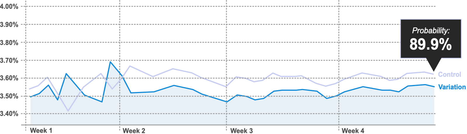
When an A/B test has been running for weeks and the result isn’t a clear win or loss, we still need to decide. Cumulative conversion rates show reward; what’s often missing is a view of risk. Expected Loss (from Chris Stucchio’s work for VWO) estimates the risk of choosing one variant over another—the lower the expected loss for a variant, the better. Showing both reward (e.g. conversion rates over time) and risk (expected loss over time) gives decision-makers a fuller picture and can shorten runtimes, especially for de-risk experiments.
The article walks through calculating Expected Loss in Python (Jupyter): load visits and conversions for control and variation; compute conversion rates; use beta distributions (via scipy.stats.beta) to generate random samples from the posterior for each variant; for each pair of samples, take the positive part of (variation − control) or (control − variation); average to get Expected Loss for each variant. With many samples (e.g. 10k+), the mean Expected Loss per variant is stable. Plotting cumulative Expected Loss over time shows when the “risk” story is stable. Suggested rules: e.g. probability of best ≥ 90%, stable expected loss lines, and seven days without the lines crossing. The dual view of risk and reward makes it easier to call results earlier and communicate with stakeholders.